Deep Learning with PyTorch: A 60 Minute Blitz 自学笔记
Tensor
张量是一种特殊的数据结构,与数组和矩阵非常相似。在PyTorch中,我们使用张量对模型的输入和输出以及模型的参数进行编码
张量类似于NumPy的ndarray,除了张量可以在GPU或其他专用硬件上运行以加速计算
1 | import torch |
Tensor Initialization
- 张量可以通过多种方式初始化
- 张量可以直接从数据中创建。数据类型是自动推断的。torch.tensor(data)
1
2data = [[1, 2], [3, 4]]
x_data = torch.tensor(data) - 张量可以从NumPy中的arrays创建,反之亦然。torch.from_numpy(np_array)
1
2np_array = np.array(data)
x_np = torch.from_numpy(np_array) - 从另一个张量,新张量将保留参数张量的属性(形状、数据类型)。torch.ones_like(tensor,type) & torch.rand_like(tensor,type)
1
2
3
4
5
6
7
8
9
10
11
12
13
14
15
16
17
18
19
20
21
22x_ones = torch.ones_like(x_data)
# retains the properties of x_data
# torch.ones_like 是 PyTorch 中的一个函数
# 它根据给定的张量(tensor)创建一个与其形状、数据类型相同的新张量
# 并且所有元素的值都为1
print(f"Ones Tensor: \n {x_ones} \n")
x_rand = torch.rand_like(x_data, dtype=torch.float)
# overrides the datatype of x_data
# torch.rand_like 是 PyTorch 中的一个函数
# 它根据给定的张量(tensor)创建一个与其形状和数据类型相同的新张量
# 其中元素是从均匀分布([0, 1))中随机采样的浮点数
print(f"Random Tensor: \n {x_rand} \n")
out:
Ones Tensor:
tensor([[1, 1],
[1, 1]])
Random Tensor:
tensor([[0.8823, 0.9150],
[0.3829, 0.9593]]) - 随机或恒定值,用shape决定输出张量的维数。(shape)
1
2
3
4
5
6
7
8
9
10
11
12
13
14
15
16
17
18
19
20
21
shape = (2, 3,)
rand_tensor = torch.rand(shape)
ones_tensor = torch.ones(shape)
zeros_tensor = torch.zeros(shape)
print(f"Random Tensor: \n {rand_tensor} \n")
print(f"Ones Tensor: \n {ones_tensor} \n")
print(f"Zeros Tensor: \n {zeros_tensor}")
out:
Random Tensor:
tensor([[0.3904, 0.6009, 0.2566],
[0.7936, 0.9408, 0.1332]])
Ones Tensor:
tensor([[1., 1., 1.],
[1., 1., 1.]])
Zeros Tensor:
tensor([[0., 0., 0.],
[0., 0., 0.]])
- 张量可以直接从数据中创建。数据类型是自动推断的。torch.tensor(data)
Tensor Attributes
- 张量属性描述了它们的形状、数据类型以及存储它们的设备。tensor.shape() & tensor.dtype() & tensor.device()
1 | tensor = torch.rand(3, 4) |
Tensor Operations
- 张量操作包括转置、索引、切片、数学运算、线性代数、随机采样等。每一个都可以在GPU上运行(通常比在CPU上运行速度更快)。torch.cuda.is_available() & tensor.to(‘cuda’)
1 | # We move our tensor to the GPU if available |
- 标准numpy类索引和切片:tensor[:,n] & tensor[n,:]
1 | tensor = torch.ones(4, 4) |
- 连接张量:使用torch.cat沿给定维度连接一系列张量。另请参见torch.stack,与torch.cat略有不同
1 | t1 = torch.cat([tensor, tensor, tensor], dim=1) |
- 乘以张量:* & @ & tensor.mul(tensor) & torch.matmul(tensor1, tensor2)
1 | # This computes the element-wise product |
- In-place operation(““):x.copy(y), x.t_(), x.add(n) will change x.
1 | print(tensor, "\n") |
- In-place operation 可以节省一些内存,但在计算导数时可能会出现问题,因为会立即丢失历史记录。因此,不鼓励使用它们
Bridge with NumPy
- CPU上的tensor和NumPy数组上的张量可以共享它们的底层内存位置,改变一个就会改变另一个
Tensor to NumPy array
- t.numpy()
1 | t = torch.ones(5) |
NumPy array to Tensor
- torch.from_numpy(n)
1 | n = np.ones(5) |
A Gentle Introduction to torch.autograd
- torch.autograd是PyTorch的自动微分引擎,为神经网络训练提供动力
Background
神经网络(NN)是对某些输入数据执行的嵌套函数的集合。这些函数由参数(由权重和偏差组成)定义,这些参数在PyTorch中存储在张量中
训练神经网络分为两个步骤:
- 正向传播:在正向传播中,神经网络对正确的输出做出最佳预测。它通过每个函数运行输入数据来进行猜测
- 反向传播:在反向传播中,神经网络根据其猜测的误差按比例调整其参数。它通过从输出向后遍历,收集误差相对于函数参数(梯度)的导数,并使用梯度下降优化参数来实现这一点
Usage in PyTorch
- 例子:我们从torchvision加载一个预训练的resnet18模型。我们创建了一个随机数据张量来表示具有3个通道、高度和宽度为64的单个图像,并将其相应的标签初始化为一些随机值。预训练模型中的标签具有形状(1,1000)
1 | import torch |
Differentiation in Autograd
- autograd如何收集梯度?
1 | import torch |
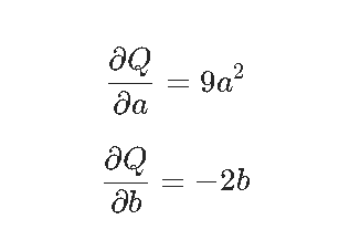
1 | # 调用.backward()时,autograd会计算这些梯度并将其存储在相应张量的.grad属性中 |
Optional Reading - Vector Calculus using autograd
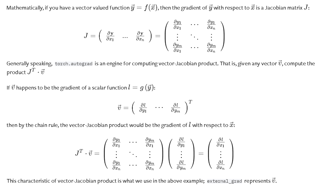
Computational Graph
autograd在由Function对象组成的有向无环图(DAG)中记录数据(张量)和所有执行的操作(以及由此产生的新张量)。在这个DAG中,叶子是输入张量,根是输出张量。通过从根到叶跟踪此图,您可以使用链式规则自动计算梯度
In a forward pass, autograd does two things simultaneously:
- 运行所请求的操作以计算结果张量
- 在DAG中保持操作的梯度函数
The backward pass kicks off when .backward() is called on the DAG root. autograd then:
- 根据每个.grad_fn计算梯度
- 将它们累积在各自张量的.grad属性中
- 使用链式规则,一直传播到叶张量
DAG的可视化表示。在图中,箭头指向正向传递的方向。节点表示正向传递中每个操作的反向函数。蓝色的叶节点表示我们的叶张量a和b
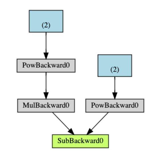
DAGs在PyTorch中是动态的。每次.backward()调用后,autograd都会开始填充一个新的图
torch.autograd跟踪所有requires_grad标志设置为True的张量上的操作。对于不需要梯度的张量,将此属性设置为False会将其从梯度计算DAG中排除
1 | x = torch.rand(5, 5) |
- 在神经网络中,不计算梯度的参数通常被称为冻结参数。在微调中,我们冻结了大部分模型,通常只修改分类器层以对新标签进行预测
1 | from torch import nn, optim |
Neural Networks
神经网络可以使用 torch.nn 包来构建
在了解了 autograd 之后,nn 依赖于 autograd 来定义模型并对其进行微分
一个 nn.Module 包含层,以及一个返回输出的 forward(input) 方法
例如这个用于分类数字图像的神经网络:
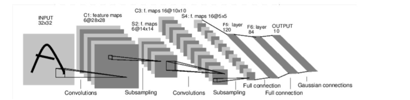
这是一个简单的前馈神经网络:它接收输入,将输入通过若干层依次传递,最后给出输出
神经网络的典型训练过程如下:
- 定义神经网络:定义具有一些可学习参数(或权重)的神经网络。
- 遍历输入数据集:对输入数据集进行迭代。
- 通过网络处理输入:将输入数据通过网络传递。
- 计算损失:计算损失(输出与正确值之间的差距)。
- 反向传播梯度:将梯度传播回网络的参数中。
- 网络权重:通常使用简单的更新规则来更新网络权重:weight = weight - learning_rate * gradient
Define the network
- 定义神经网络:
1 | import torch |
只需要定义 forward 函数,backward 函数(用于计算梯度)会通过 autograd 自动定义
可以在 forward 函数中使用任何 Tensor 操作
模型的可学习参数可以通过 net.parameters() 返回
1 | params = list(net.parameters()) |
让我们尝试一个随机的 32x32 输入
注意:这个网络(LeNet)期望的输入大小是 32x32。要在 MNIST 数据集上使用此网络,请将数据集中的图像调整为 32x32 的大小
1 | input = torch.randn(1, 1, 32, 32) |
将所有参数的梯度缓冲区清零,并使用随机梯度进行反向传播:
torch.nn 仅支持小批量(mini-batch)。整个 torch.nn 包只支持输入为小批量样本,而不支持单个样本
例如,nn.Conv2d 需要一个形状为 nSamples x nChannels x Height x Width 的四维张量作为输入
如果只有一个单个样本,可以使用 input.unsqueeze(0) 添加一个伪批量维度
1 | net.zero_grad() |
- summary:
- torch.Tensor - 一种多维数组,支持自动求导操作,如 backward()。它还保存了相对于该张量的梯度
- nn.Module - 神经网络模块。封装参数的便捷方式,提供了将参数移动到 GPU、导出、加载等辅助功能
- nn.Parameter - 一种特殊的张量(Tensor),当作为属性分配给 Module 时,会自动注册为参数
- autograd.Function - 实现了自动求导操作的前向和反向定义。每个张量操作至少会创建一个 Function 节点,该节点连接到创建该张量的函数,并编码其历史记录
Loss Function
损失函数 接收一对输入(输出值 output 和目标值 target),并计算一个值,用于估计输出值与目标值之间的差距
在 nn 模块中有多种不同的损失函数。一个简单的损失函数是:nn.MSELoss,它计算输出值与目标值之间的均方误差
1 | output = net(input) |
如果沿着损失函数的反向传播方向(通过其 .grad_fn 属性)追踪,您会看到一个类似以下的计算图:
input -> conv2d -> relu -> maxpool2d -> conv2d -> relu -> maxpool2d
-> flatten -> linear -> relu -> linear -> relu -> linear
-> MSELoss
-> loss当调用 loss.backward() 时,整个计算图会相对于神经网络的参数进行微分,并且图中所有 requires_grad=True 的张量都会将其梯度累加到 .grad 属性中
为了更直观地理解,让我们一步步反向追踪:
1 | print(loss.grad_fn) # MSELoss |
Backprop
要反向传播误差,我们只需要调用 loss.backward()。但在此之前需要清除现有的梯度,否则梯度会累积到现有的梯度上。
现在我们将调用 loss.backward(),并观察 conv1 的偏置梯度在反向传播前后的变化:
1 | net.zero_grad() # zeroes the gradient buffers of all parameters |
Update the weights
- 在实践中使用的最简单的更新规则是随机梯度下降法(Stochastic Gradient Descent, SGD):
1 | weight = weight - learning_rate * gradient |
- 其他梯度下降的方法例如 SGD、Nesterov-SGD、Adam、RMSProp 等。为了实现这一点,工具包:torch.optim,它实现了所有这些方法
1 | import torch.optim as optim |
- 需要注意的是,必须使用 optimizer.zero_grad() 手动将梯度缓冲区清零。这是因为梯度会累积,正如在反向传播部分所解释的那样
Training a Classifier
What about data?
通常当需要处理图像、文本、音频或视频数据时,可以使用标准的 Python 包将数据加载到 NumPy 数组中。然后可以将该数组转换为 torch.*Tensor:
- 对于图像,可以使用诸如 Pillow 和 OpenCV 等包。
- 对于音频,可以使用诸如 scipy 和 librosa 等包。
- 对于文本,可以使用基于原始 Python 或 Cython 的加载方式,或者使用 NLTK 和 SpaCy 等工具。
对于视觉任务, torchvision 包提供了常见数据集(如 ImageNet、CIFAR10、MNIST 等)的数据加载器,以及针对图像的数据转换工具,例如 torchvision.datasets 和 torch.utils.data.DataLoader。
在本教程中,将使用 CIFAR10 数据集。它包含以下类别: ‘airplane’, ‘automobile’, ‘bird’, ‘cat’, ‘deer’, ‘dog’, ‘frog’, ‘horse’, ‘ship’, ‘truck’
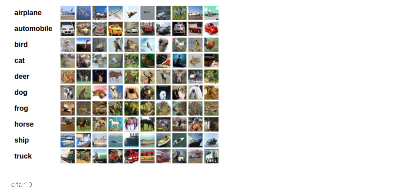
- CIFAR-10 中的图像尺寸为 3x32x32,即 32x32 像素大小的 3 通道彩色图像
Training an image classifier
- 实现步骤:
- 使用 torchvision 加载并标准化 CIFAR10 的训练和测试数据集
- 定义一个卷积神经网络(Convolutional Neural Network, CNN)
- 定义一个损失函数
- 在训练数据上训练网络
- 在测试数据上测试网络
Load and normalize CIFAR10
使用torchvision加载 CIFAR10
torchvision 数据集的输出是范围在 [0, 1] 的 PILImage 图像。我们将它们转换为范围在 [-1, 1] 的归一化张量
注意:如果在 Windows 上运行并遇到 BrokenPipeError 错误,可以尝试将 torch.utils.data.DataLoader() 的 num_worker 参数设置为 0
1 | import torch |
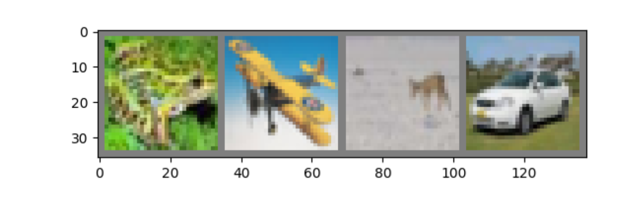
- 可以通过如下方法打印训练图片:
1 | import matplotlib.pyplot as plt |
Define a Convolutional Neural Network
- 将之前 神经网络部分 的神经网络代码复制过来,并修改它以处理 3 通道图像(而不是原本定义的 1 通道图像)
1 | import torch.nn as nn |
Define a Loss function and optimizer
- 使用Classification Cross-Entropy loss and SGD with momentum
1 | import torch.optim as optim |
Train the network
- 只需要遍历数据迭代器,将输入数据传递给网络并进行优化即可:
1 | for epoch in range(2): # loop over the dataset multiple times |
- 可以通过下面的代码保存模型:
1 | PATH = './cifar_net.pth' |
Test the network on the test data
我们已经让网络在训练数据集上训练了 2 轮。但我们需要检查网络是否学到了任何东西
通过预测神经网络输出的类别标签,并将其与真实标签进行比较来验证这一点。如果预测正确,我们将该样本添加到正确预测的列表中
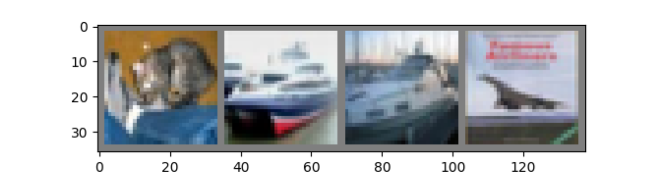
第一步:从测试集中显示一张图像,以便熟悉数据
1 | dataiter = iter(testloader) |
- 加载之前保存的模型(注意:在这里保存和重新加载模型并不是必需的,我们只是为了演示如何操作)
1 | net = Net() |
- 现在让我们看看神经网络认为上述示例属于哪些类别,输出是 10 个类别的值。某个类别的值越高,网络就越认为图像属于该特定类别
1 | outputs = net(images) |
- 神经网络在整个数据集上的操作:
1 | correct = 0 |
看起来比随机猜测要好得多,随机猜测的准确率是 10%(从 10 个类别中随机选择一个类别)。看来网络确实学到了一些东西
下面来看看神经网络在各个类别上的预测
1 | # prepare to count predictions for each class |
Training on GPU
就像将张量(Tensor)转移到 GPU 上一样,也可以将神经网络转移到 GPU 上
首先,如果我们有可用的 CUDA 设备,我们将设备定义为第一个可见的 CUDA 设备
1 | device = torch.device('cuda:0' if torch.cuda.is_available() else 'cpu') |
本节的其余部分假设 device 是一个 CUDA 设备。然后,这些方法会递归地遍历所有模块,并将它们的参数和缓冲区转换为 CUDA 张量
请记住还需要在每一步将输入和目标数据也发送到 GPU:
1 | net.to(device) |