计算机视觉 22 Image Generation
自回归模型(Autoregressive Models)
显式概率密度估计(Explicit Density Estimation: Autoregressive Models)
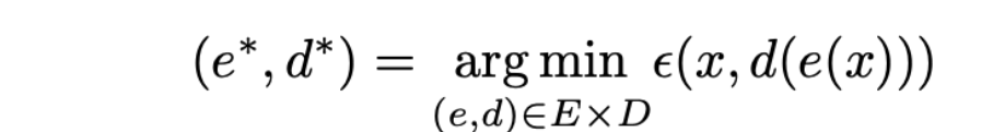
目标:得到显式函数p(x) = f(x,W)
给定数据集x(1),x(2),…,x(n),通过极大似然估计来训练模型:

- Autoregressive Models:
- 假设每个 x 由多个子部分(维度)组成:x=(x1,x2,…,xT)
- 使用链式法则分解概率表达式:

- 通过将上述方程代入损失函数来求 W∗。给定历史作为已知条件来预测下一个
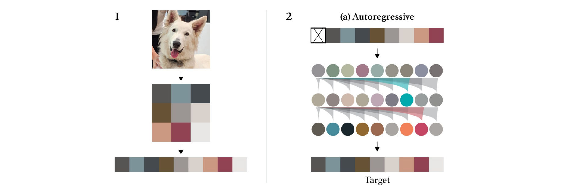
PixelCNN and PixelRNN
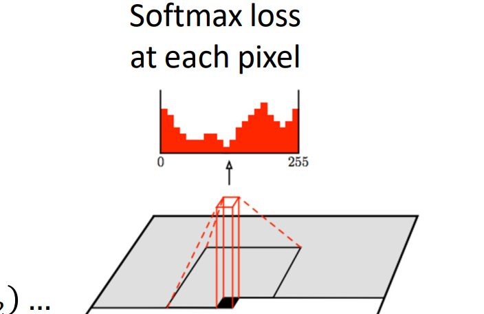
从左上角开始,一次生成一个图像像素,逐像素生成
使用 RNN或CNN计算每个像素的概率,该概率取决于状态和从左侧和上方的 RGB值:

- 在每个像素处,预测红色,然后预测蓝色,然后预测绿色:softmax到[0,1,…,255]
Generative Pretraining from Pixels
- 使用自回归模型的Transformer:
变分自编码器(Variational Autoencoder)
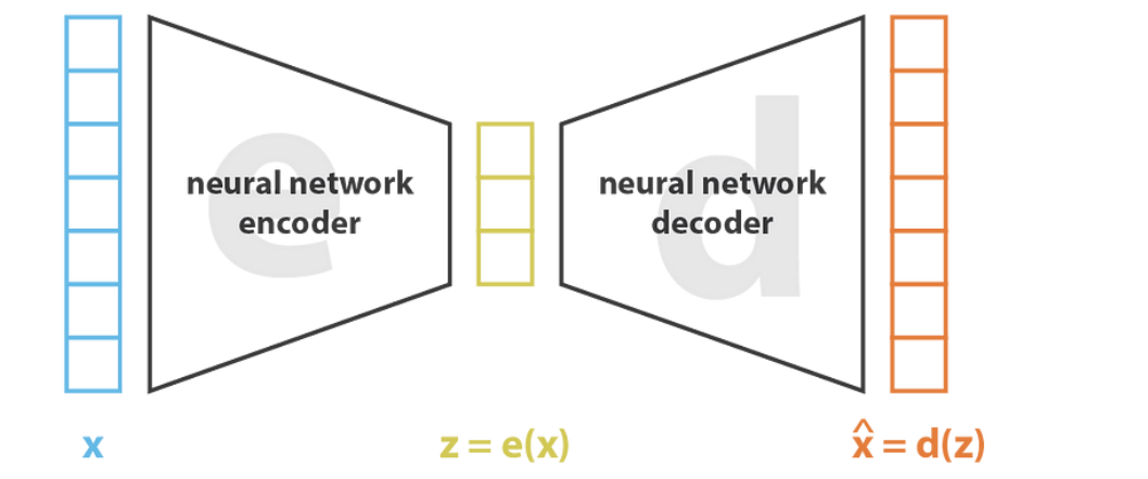
Autoencoder
Autoencoder:编码器压缩数据(CNN,降采样),解码器重构数据(上采样);通常用于未标记数据的降维
编码器 e 和解码器 d 通常是神经网络
PCA 是一种线性自动编码器:
- 其中,损失函数ε可以是 L2 损失或交叉熵损失。希望能够恢复原状,和x进行比较
- Autoencoder(黄)相比于PCA(蓝)更结构化,效果更好
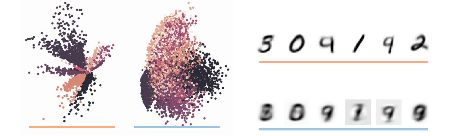
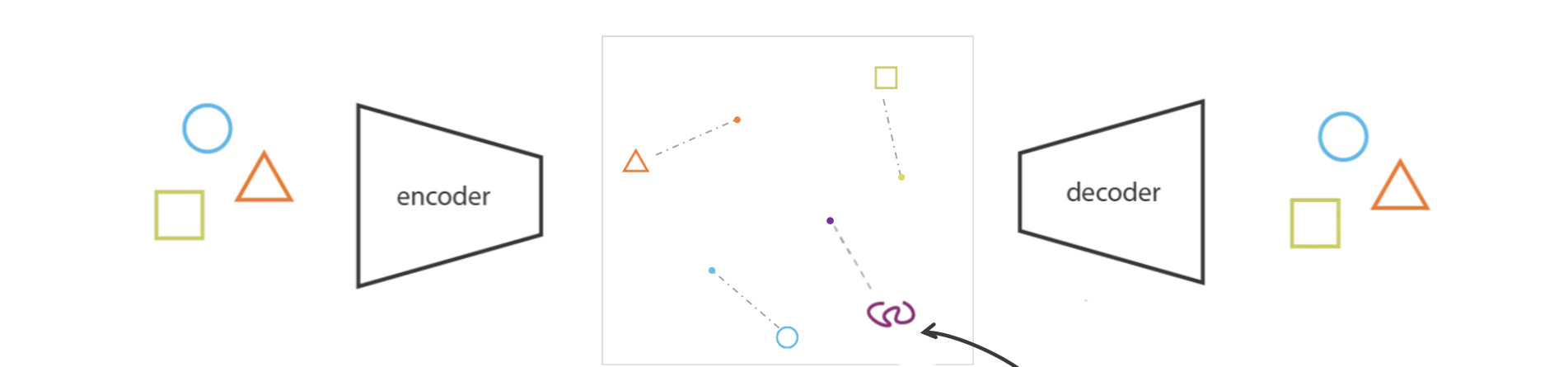
Autoencoder is not a Generative Model
- 如果没有适当的正则化,来自潜在空间的样本可能毫无意义。由于其对隐空间无约束,所以若不是词典内的输入,可能导致不合理输出(位于中间地带)
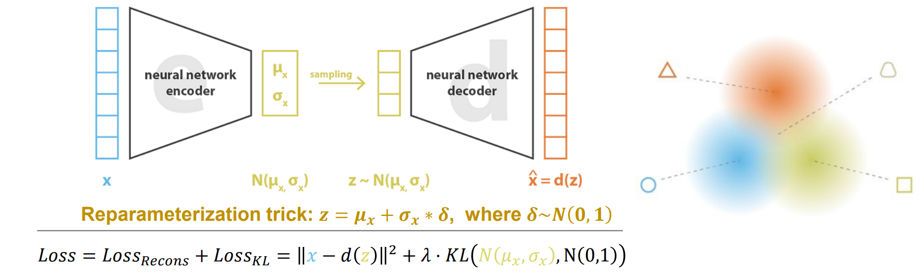
Reparameterization trick: 𝒛 = 𝝁𝒙 + 𝝈𝒙 ∗ 𝜹, where 𝜹~𝑵(𝟎,𝟏),采样不可微而z可微
经过Reparameterization trick后预测不是点而是预测分布,使得隐空间的区域都有一定覆盖,可以重建出过渡体
𝜹是噪音,可能导致坍缩,且隐空间中间缝隙会增大,所以需要进行KL loss正则化使得𝝁𝒙=0,σx=1靠拢:
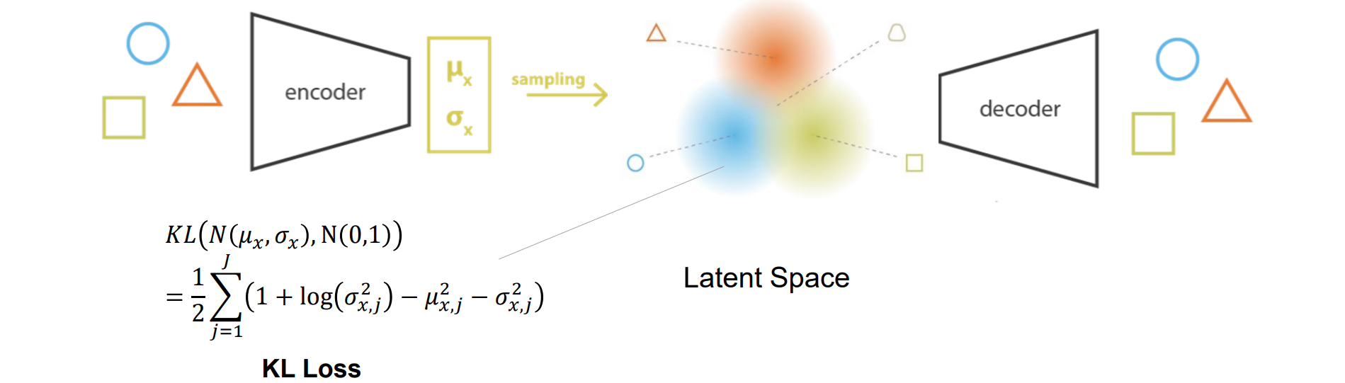
- 变分自动编码器:自动编码器 + 潜在空间具有良好的特性,可以实现生成过程
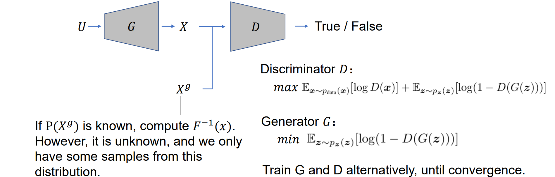
Generative Adversarial Network(GAN)
- 随机数发生器(Generate uniform random numbers),线性同余:

- 其他分布:𝑋 = 𝐹^−1 (U),其中F(X)是X的累积分布
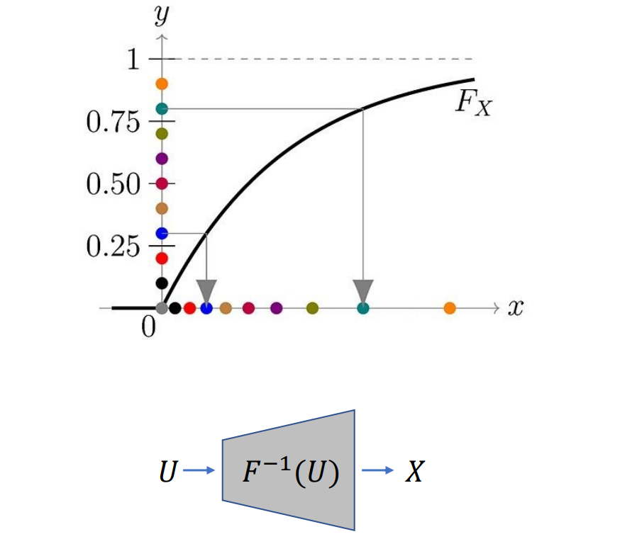
GAN:用神经网络拟合F(X)反函数:
- G是生成器:生成样本X和真实样本X(g)尽可能一样,用神经网络完成
- D是判别器:通过二分类使X置为0,X(g)置为1
- 训练G和D直到判别器的正确率均为1/2说明已经分别不出来生成的X和真实的X(g)(平衡位置)
如果 P(Xg) 已知,则计算 F^−1(x)。但是它是未知的,只有来自此分布的一些样本
GAN:
1 | import torch |
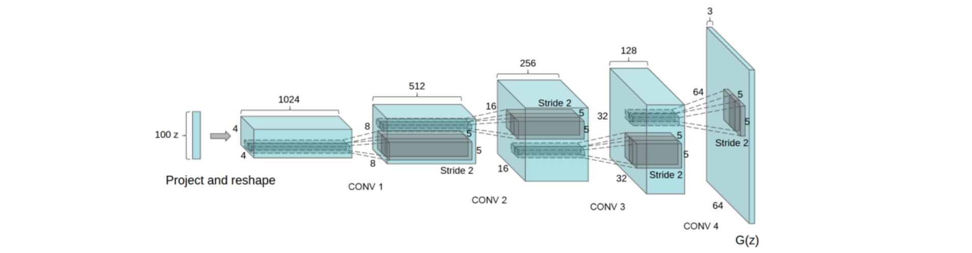
The Generator of DCGAN
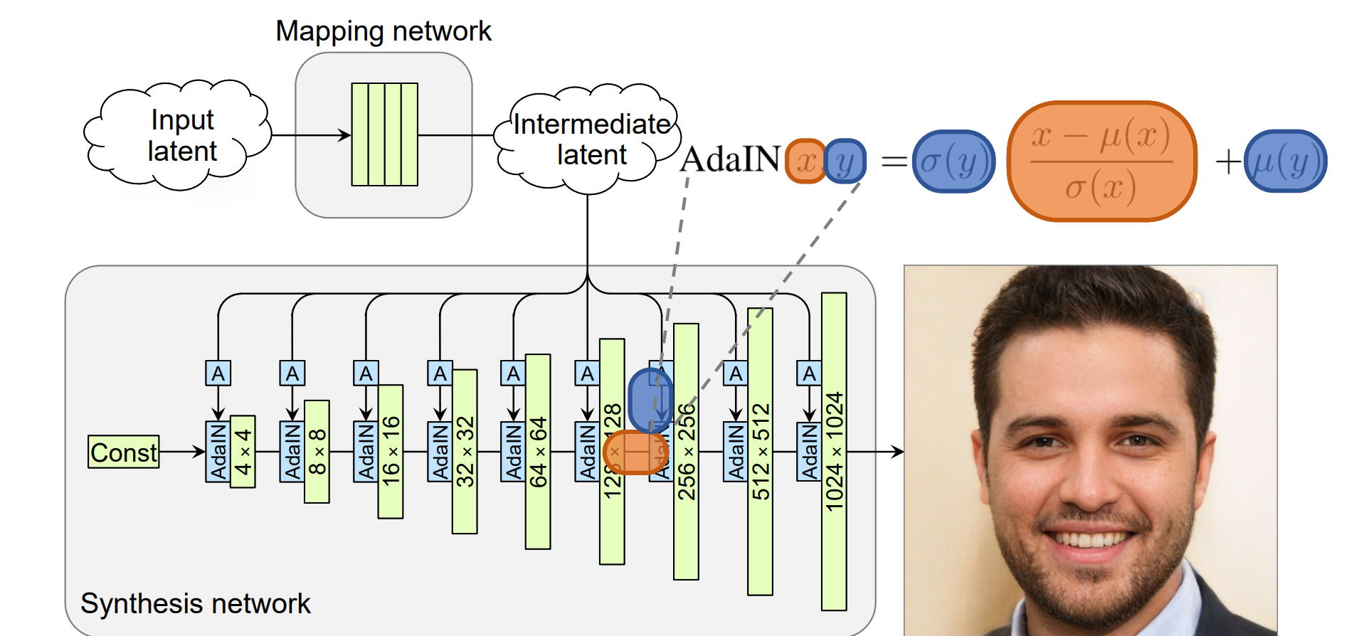
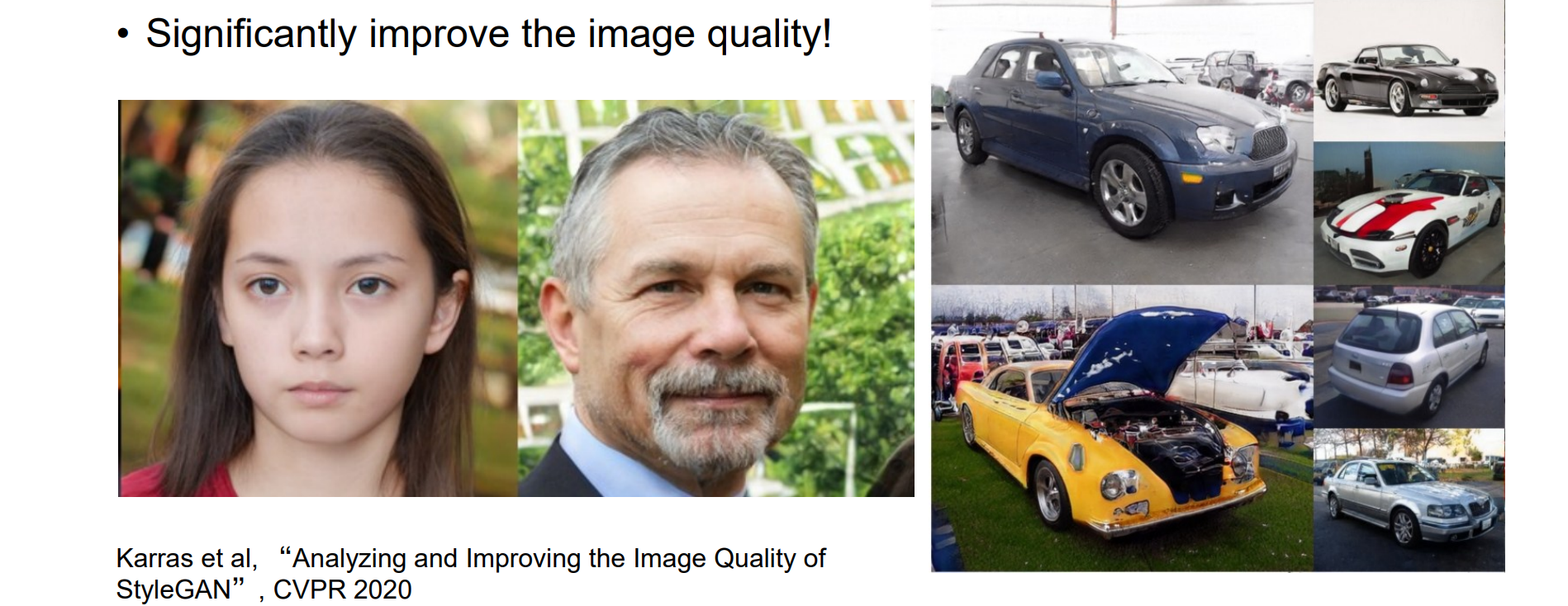
StyleGAN
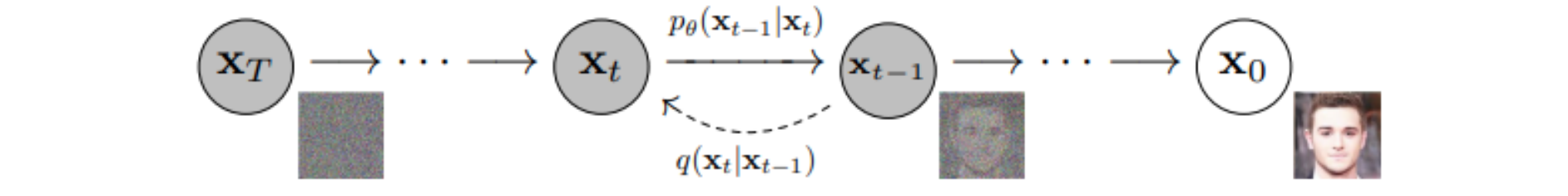
Diffusion Models
- Diffusion Models通过前向过程和逆向过程来制造仿真:
- 前向过程:逐渐添加噪声,直到得到高斯噪声
- 逆向过程:逐渐去除噪点,直到我们得到干净的图像
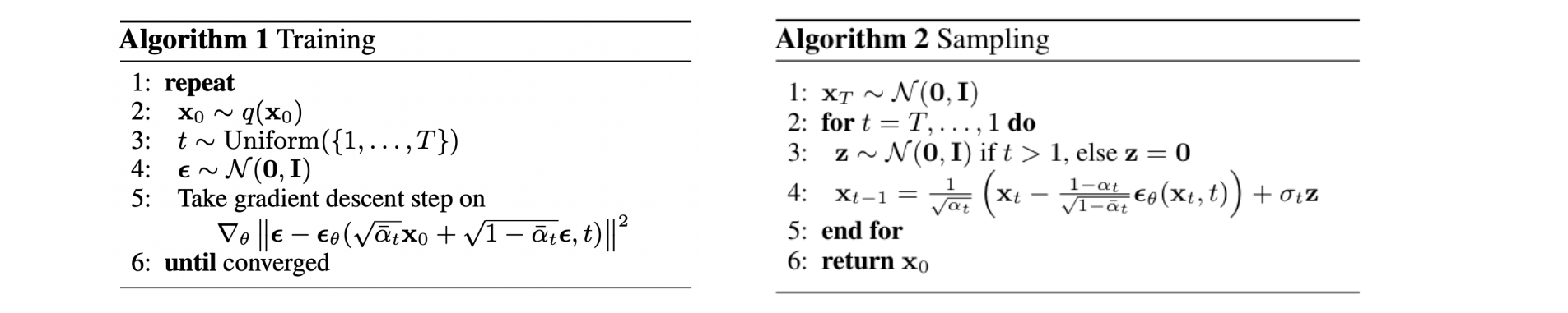
Forward Process
- 马尔可夫链,与历史状态无关;当 αt 增加时,xt 变为高斯噪声:

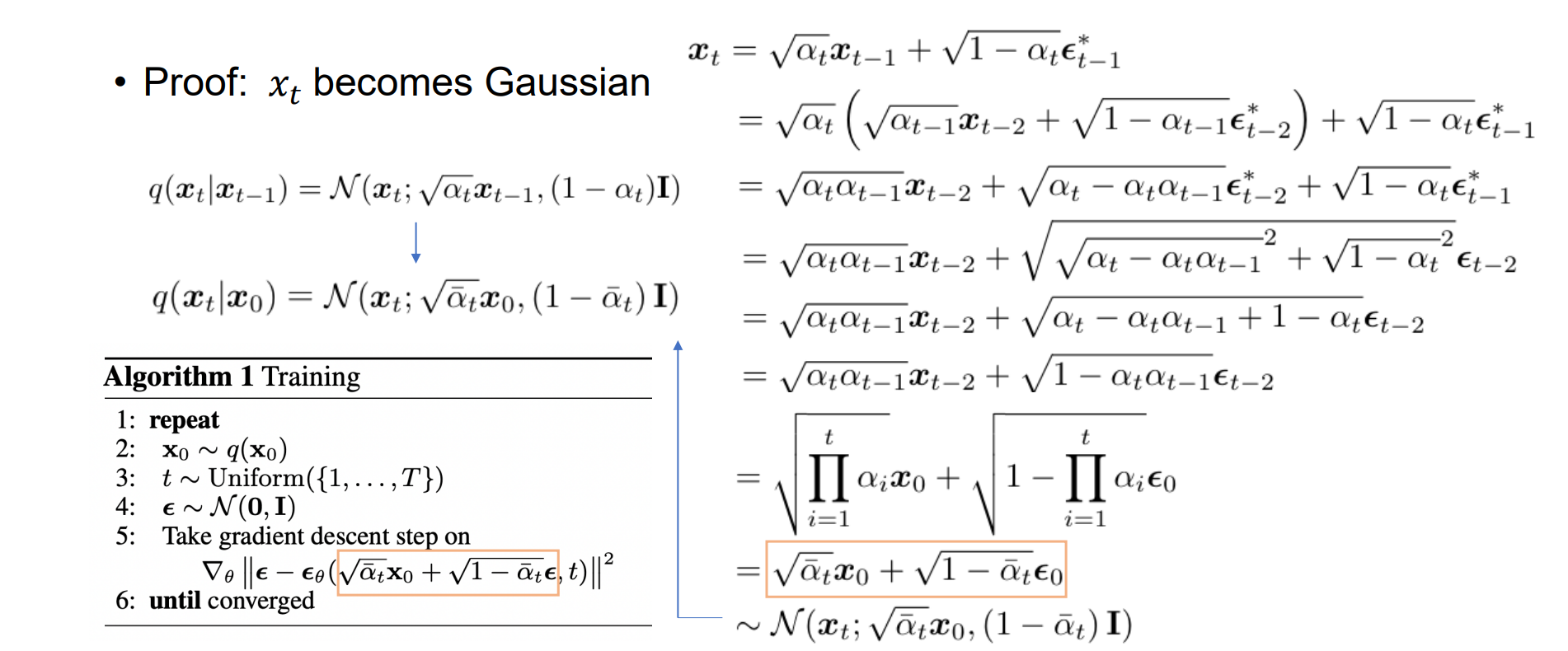
Inverse Process
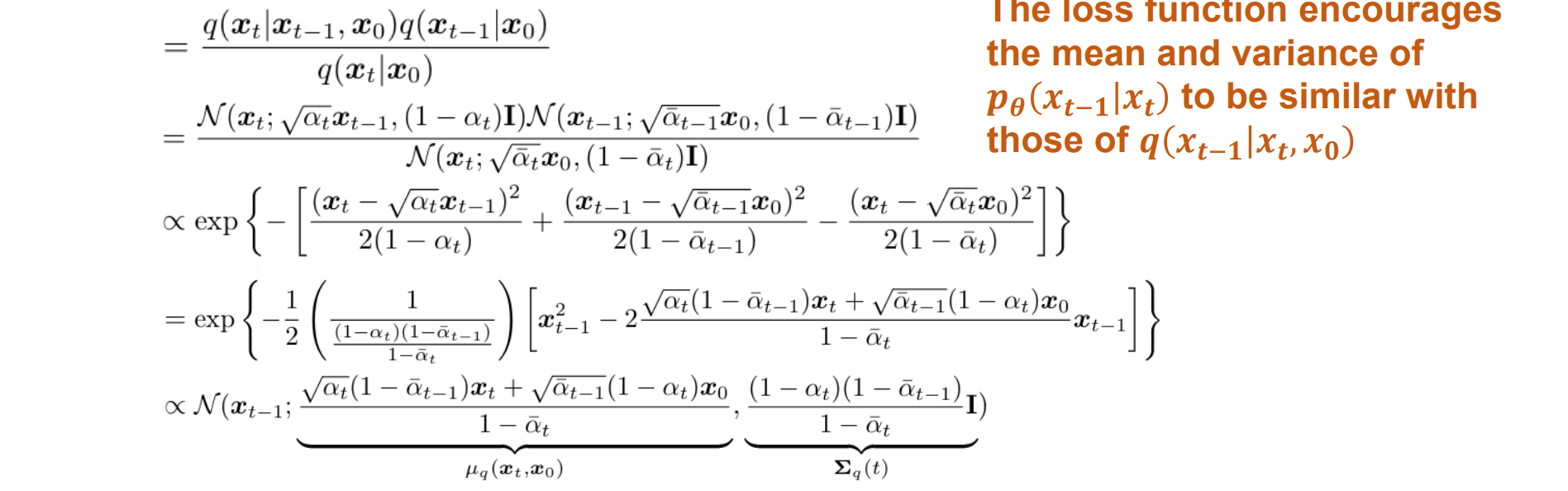
目标:估计q(xt−1|xt)当 T 很大时,假设它是高斯的
关键观察:q(xt−1|xt,x0)也是高斯的
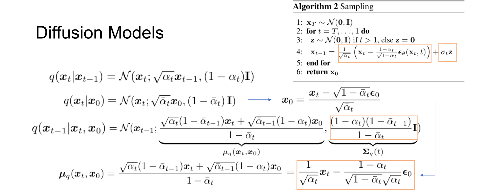
- Diffusion Models(DDPM):
1 | import torch |
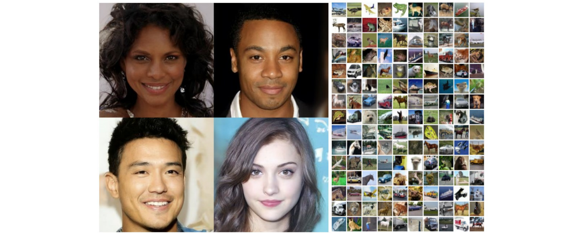
DDPM 2020
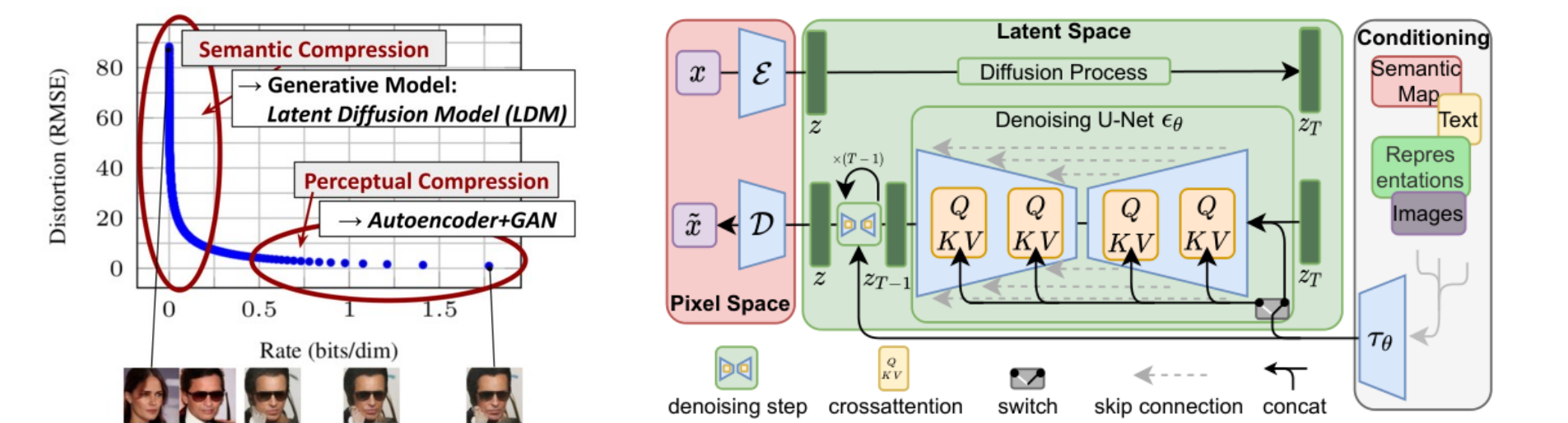
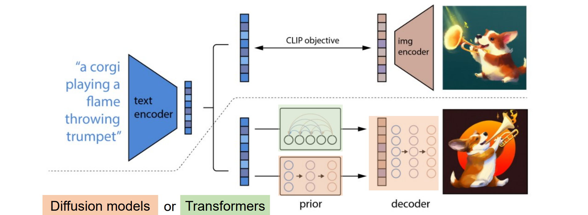
DALL·E 2022
Stable Diffusion 2022